Final Project

As a culmination to the Geography 390 course I have created two maps displaying different geographic phenomena. These maps adhere to correct cartographic convention in all forms including color scheme, labeling/text placement, map elements, data classification and layout. The first map is largely qualitative and meant to inform map users of extreme precipitation values in Cascade Mountain region of the state of Washington. The second map is more quantitative. This map conveys the racial makeup of the Chicago Metropolitan Area of the state of Illinois. Using a bivariate standard, the map shows both percentage of non-white population in this region using a choropleth mapping technique, as well as the proportion of each race in bar graph form. Both of these maps are meant to be user friendly and largely informative for an interested audience. Clarity, conciseness, and simplicity were the goals in designing these maps to portray the information as efficiently and effectively as possible. The two maps I created are displayed below:

Map 1:

Map 2:

Lab 7: Bivariate/Multivariate Mapping

Map I: Pie Chart

The purpose of the map is to portray the composition of races in Idaho counties excluding the white population. The pie charts unique to each county exhibit what races exist by proportion of the whole. This kind of map is easy to interpret as long as the legend is clearly labeled.

Pie chart maps are very user friendly and map readers should be able to extract the information portrayed with little difficulty. However, there are several limitations to this kind of mapping. When the variable chart size option is selected the user cannot manually set the max size of the pie charts. This can cause several problems: the minimum chart size must be set to where the user can read it, but if it gets too large the maximum sized charts become crowded and the map looks cluttered and unorganized. Color schemes are also difficult to choose to where the largest proportions of the pie charts do not have a color that is too overwhelming. It is much easier to manually choose the colors to best portray the information. I chose lighter shades of colors for the most dominant proportions and bright colors for the smallest so that they could be seen in contrast. This seemed to solve the problem.

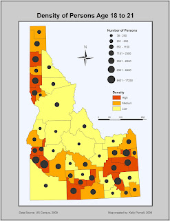
Map II: Bivariate Map

The purpose of this map was to portray the population density of persons age 18 to 21. This was done by selecting both the attribute Age 18-21 and Density_gp. Density_gp was a background choropleth map depicting whether the density of this age group was high, medium, or low within Idaho counties. The attribute Age 18-21 is raw data. This was mapped using proportional symbols to portray the total number of this age group in each Idaho county. This kind of map is fairly easy to interpret with the proper legend and a well chosen color scheme. The map reader should be able to evaluate which counties have the highest population density of the chosen age group with ease. The color scheme of the choropleth map was chosen for lightness as well as change in hue so that counties with the highest value showed up in red (dark and warm), medium values showed up in orange (medium hue), and low lowest values were light yellow (warm and muted). This was chosen for qualitative purposes as it is easy to extract the information of the map.

There were several difficulties in this bivariate mapping exercise. Choosing the data classification method of the raw data was not the easiest task. The classification needed to be show the greatest differentiation in symbol size for the proportional symbology. I ended up choosing seven classes using the Natural Breaks method as this seemed to best capture the variation in quantities of the population age 18 to 21.

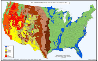
Map of the Week: USDA Soils Map

This map is the USDA soils map. The point of the map is to portray where the most drought occurs. As a thematic map, this is well done and accurately and effectively portrays the information and purpose.

Lab 6: IDW and Kriging Interpolation

Part I: Inverse Distance Weighted (IDW) Interpolation


The map shows the annual precipitation in Idaho. This is an Isarithmic map using Inverse Distance Weighted (IDW) interpolation to find the best estimation for isobars (contours) between weather stations where actual information exists. This was a decent method and had a minimal RMSE. The IDW interpreted somewhat detailed variations in temperature throughout the state.








Part II: Kriging Interpolation

This map also shows the annual precipitation in Idaho. This is an Isarithmic map using Kriging interpolation to find the best estimation for isobars (contours) between weather stations where actual information exists. The best statistics were obtained through the Spherical Kriging model which shows a progressive decrease of spatial autocorrelation (equivalently, an increase of semivariance) until some distance beyond which autocorrelation is zero.








Discussion:

The maps using IDW interpolation and Kriging interpolation look very similar. However at a closer inspection it can be seen that the contours that were interpolated for the IDW method represent a more detailed interpretation of the estimated values between the precipitation grid points on the map. It seems that the IDW picked up on higher level of variation in the points. This map used 15 neighbors and the optimal power to determine the best values for the contours. The Kriging Map, though similar is shows much less variation in the contours and did not pick up on small peaks in the precipitation variation. Despite this the max and min values for annual precipitation are very similar.

Map of the Week: Elevation map of Salem, OR

I chose this map because I wanted to show a relatively bad example of a raster elevation map. The map is of the city of Salem, Oregon and is meant to represent elevation values as well as city features. However, at first glance one might think this is a map of ocean depths. The qualitative value of the map is poorly done. Shades of blue were not a great choice to protray elevation, especially considering that Salem is not near the coast. I thought this was a good example of what not to do when creating an elevation map.

source: http://www.cityofsalem.net/Departments/InformationTechnology/GIS/Pages/ElevationMaps.aspx

Lab 5 Maps

Dot Map: I had a few difficulties with this map in deciding what value to set the dots at. I experimented with several different values. Due to the high number of persons within the age group of 22 to 29 I decided to set the dot value at 100 persons per dot. This value seemed to have the best density when the dots coalesced without overlapping too much. The rest of the map I adhered as much as possible to cartographic convention on map elements and layout.










Graduated Symbols: I really didn’t know what to choose for symbol size. I wanted to portray as much of the population change as possible. Since the populations ranged 770,000 to over 9 million I wanted to show the range. I experimented with different values using manual breaks in the classification and also the symbol size max and mins until I felt I had a well balanced map. I chose the colors according to the lab instructions which seemed to work well, and tried to maximize the use of white space.






Proportional Symbols: I had a lot of problems with this map and I’m really not satisfied with the way it turned out. The I chose the attribute, average household size, because it seemed to be one of the only ones that didn’t need to be normalized in order to work. I used a house as the symbol for a more qualitative use of the map. My legend did not work well and I had to convert it to graphics and scale the symbols manually in order to have a proper legend.

Map of the Week: I chose this map because I thought it was an interesting example of thematic mapping. The map is a 3-D representation of population change in Canada by province. Its both qualitative and quantitative. its well balanced with good use of color and map element placement. Source: geodepot.statcan.ca

Lab 1: Qualitative Map

Qualitative:

The purpose of the qualitative map was to show what the dominant race was in Buffalo, New York. The data represented in this map is nominal. This is just to show where where the majority of each selected race is present. The map is effective in showing the spatial location of the data. In this map I changed some of the map elements. I added a neatline and a frameline and made the outside grey to better highlight the map. I put a frame arund the legend as well to help distinguish it from the map but without drawing too much attention. I left the colors the same as they adequately portray the data without being too eye jarring. I made the map figure itself larger to eliminate more white space.

Lab 1: Quantitative Map

Quantitative Map:
The quantitative map shows the ratio of children age 5 to 17. The data is numerical and represents the percentage of the population that has that age range of children in each census block of Buffalo, New York. I have changed several things on this map, most notibly the color scheme. The previous color scheme was too abrasive and may be better suited for a qualitative map. There is some gradation in the redesigned map and better represents numerical data. I put in a frameline and neatline, changed the title to better represent the map and reduced the title on the legend. These make for better contrast and understanding of the data represented.

Lab 1: Nez Perce Map

Nez Perce Map:
This map represents how the Nez Perce lands have been reduced over a long period of time. The data needed to have clear contrast to better determine the change in land ownership. I didn’t change too much on this map. I changed the color of the aboriginal land from green to beige to show better background contrast from the current Nez Perce lands. I changed the legend slightly as well removed the word “Legend” to better apply cartographic convention for map elements.